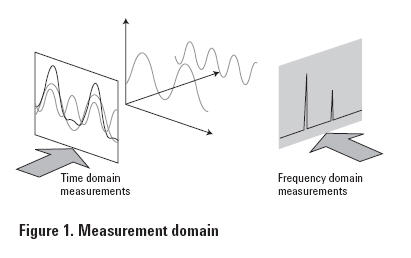
Agilent Technologies - Spectrum Analyzer Application Note 1286-1

8 Hints For Better Spectrum Analyzer Measurements

The spectrum analyzer, like an oscilloscope, is a basic tool used for observing signals. Where the oscilloscope provides a window into the time domain, the spectrum analyzer provides a window into the frequency domain, as depicted in Figure 1.

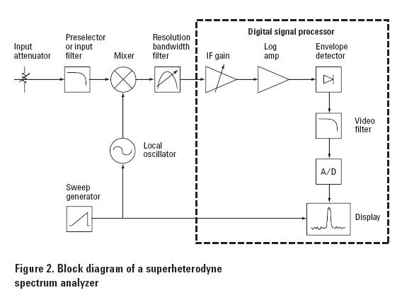
Figure 2 depicts a simplified block diagram of a swept-tuned superheterodyne spectrum analyzer.

Superheterodyne means to mix or to translate in a frequency above audio frequencies. In the analyzer, a signal at the input travels through an attenuator to limit the amplitude of the signal at the mixer, and then through a low-pass input filter to eliminate undesirable frequencies. Past the input filter, the signal gets mixed with a signal generated by the local oscillator (LO) whose frequency is controlled by a sweep generator. As the frequency of the LO changes, the signals at the output of the mixer (which include the two original signals, their sums and differences and their harmonics), get filtered by the resolution bandwidth filter (IF filter), and amplified or compressed in the logarithmic scale. A detector then rectifies the signal passing through the IF filter, producing a DC voltage that drives the vertical portion of the display. As the sweep generator sweeps through its frequency range, a trace is drawn across the screen. This trace shows the spectral content of the input signal within the selected frequency range.

When digital technology first became viable, it was used to digitize the video signal, as shown in Figure 2. As digital technology has advanced over the years, the spectrum analyzer has evolved to incorporate digital signal processing (DSP), after the final IF filter as shown by the dotted box,

to be able to measure signal formats that are becoming increasingly complex. DSP is performed to provide improved dynamic range, faster sweep speed and better accuracy. To get better spectrum analyzer measurements the input signal must be undistorted, the spectrum analyzer settings must be wisely set for application-specific measurements, and the measurement procedure optimized to take best advantage of the specifications. More details on these steps will be addressed in the hints for spectrum analysis

Hint 1. Selecting the Best Resolution Bandwidth (RBW)

The resolution bandwidth (RBW) setting must be considered when concerned with separating spectral components, setting an appropriate noise floor and demodulating a signal. When making demanding spectrum analysis measurements, spectrum analyzers must be accurate, fast and have high dynamic range. In most cases, emphasis on one of these parameters adversely impacts the others. Oftentimes, these tradeoffs involve the RBW setting. One advantage of using a narrow RBW is seen when making measurements of low-level signals. When using a narrow RBW, the displayed average noise level (DANL) of the spectrum analyzer is lowered, increasing the dynamic range and improving the sensitivity of the spectrum analyzer. In Figure 3, a -95 dBm signal is more properly resolved by changing the RBW from 100 kHz to 10 kHz.

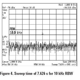
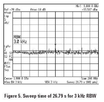
However, the narrowest RBW setting is not always ideal for spectrum analysis. For modulated signals, it is important to set the RBW wide enough to include the sidebands of the signal. Neglecting to do so will make the spectrum analysis measurement very inaccurate. Also, a serious drawback of narrow RBW settings is in sweep speed. A wider RBW setting allows a faster sweep across a given span compared to a narrower RBW setting. Figures 4 and 5 compare the sweep times between a 10 kHz and 3 kHz RBW when measuring a 200 MHz span.

It is important to know the fundamental tradeoffs that are involved in RBW selection, for cases where the user knows which measurement parameter is most important to optimize. But in cases where measurement parameter tradeoffs cannot be avoided, the modern spectrum analyzer provides ways to soften or even remove the tradeoffs. By utilizing digital signal processing the spectrum analyzer provides for a more accurate measurement, while at the same time allowing faster spectrum analysis measurements, even when using narrow RBW.

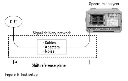
Hint 2. Improving Measurement Accuracy

Before making any spectrum analysis measurement, it is important to know that there are several techniques that can be used to improve both amplitude and frequency measurement accuracies. Available self-calibration routines will generate error coefficients (for example, amplitude changes versus resolution bandwidth), that the analyzer later uses to correct measured data, resulting in better amplitude measurements and providing you more freedom to change controls during the course of a measurement. Once the device under test (DUT) is connected to the calibrated spectrum analyzer, the signal delivery network may degrade or alter the signal of interest, which must be canceled out of the measurement as shown in Figure 6.

One method of accomplishing this is to use the spectrum analyzer’s built-in amplitude correction function in conjunction with a signal source and a power meter. Figure 7 depicts the frequency response of a signal delivery network that attenuates the DUT’s signal.

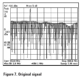
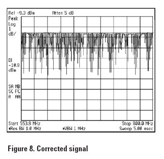
To cancel out unwanted effects, measure the attenuation or gain of the signal delivery network at the troublesome frequency points in the measurement range. Amplitude correction takes a list of frequency and amplitude pairs, linearly connects the points to make a correction “waveform,” and then offsets the input signal according to these corrections. In Figure 8, the unwanted attenuation and gain of the signal delivery network have been eliminated from the measurement, providing for more accurate amplitude measurements.

In the modern spectrum analyzer, you can also directly store different corrections for your antenna, cable and other equipment so calibration will not be necessary every time a setting is changed. One way to make more accurate frequency measurements is to use the frequency counter of a spectrum analyzer that eliminates many of the sources of frequency uncertainty, such as span. The frequency counter counts the zero crossings in the IF signal and offsets that count by the known frequency offsets from local oscillators in the rest of the conversion chain. Total measurement uncertainty involves adding up the different sources of uncertainty in the spectrum analyzer. If any controls can be left unchanged such as the RF attenuator setting, resolution bandwidth, or reference level, all uncertainties associated with changing these controls drop out, and the total measurement uncertainty is minimized. This exemplifies why it is important to know your spectrum analyzer design. For example, there is no added error when changing RBW in the high-performance spectrum analyzers that digitize the IF, whereas in others there is.

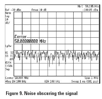
Hint 3. Optimize Sensitivity When Measuring Low-level Signals

A spectrum analyzer’s ability to measure low-level signals is limited by the noise generated inside the spectrum analyzer. This sensitivity to low-level signals is affected by the analyzer settings. Figure 9, for example, depicts   50 MHz signal that appears to be shrouded by the analyzer’s noise floor. To measure the low-level signal, the spectrum analyzer’s sensitivity must be improved by minimizing the input attenuator, narrowing down the resolution bandwidth (RBW) filter, and using a preamplifier. These techniques effectively lower the displayed average noise level (DANL), revealing the low-level signal.  

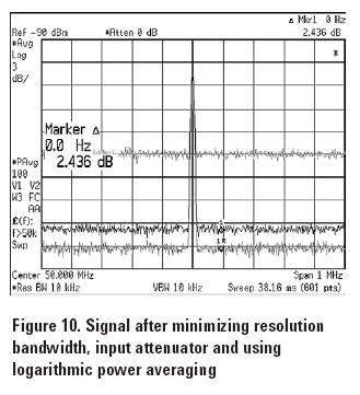
Increasing the input attenuator setting reduces the level of the signal at the input mixer. Because the spectrum analyzer’s noise is generated after the input attenuator, the attenuator setting affects the signal-to-noise ratio (SNR). If gain is coupled to the input attenuator to compensate for any attenuation changes, real signals remain stationary on the display.  However, displayed noise level changes with IF gain, reflecting the change in SNR that result from any change in input attenuator setting.  Therefore, to lower the DANL, input attenuation must be minimized.  An amplifier at the mixer’s output then amplifies the attenuated signal to keep the signal peak at the same point on the analyzer’s display. In addition to amplifying the inpu signal, the noise present in the analyzer is amplified as well, raising the DANL of the spectrum analyzer.  The re-amplified signal then passes through the RBW filter. By narrowing the width of the RBW filter, less noise energy is allowed to reach the envelope detector of the analyzer, lowering the DANL of the analyzer.  Figure 10 shows successive lowering of the DANL. The top trace shows the signal above the noise floor after minimizing resolution bandwidth and using power averaging. The trace that follows beneath it shows what happens with minimum attenuation.  The third trace employs logarithmic power averaging, lowering the noise floor an additional 2.5 dB, making it very useful for very sensitive measurements.

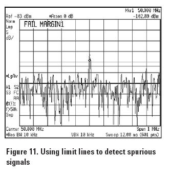
To achieve maximum sensitivity, a preamplifier with low noise and high gain must be used. If the gain of the amplifier is high enough (the noise displayed on the analyzer increases by at least 10 dB when the preamplifier is connected), the noise floor of the preamplifier and analyzer combination is determined by the  noise figure of the amplifier.  In many situations, it is necessary to measure the spurious signals of the device under test to make sure that the signal carrier falls within a certain amplitude and frequency “mask”. Modern spectrum analyzers provide an electronic limit line capability that compares the trace data to a set of amplitude and frequency (or time) parameters. When the signal of interest falls within the limit line boundaries, a display indicating PASS MARGIN or PASS LIMIT (on Agilent analyzers) appears. If the signal should fall out of the limit line boundaries, FAIL MARGIN or FAIL LIMIT appears on the display as shown on Figure 11 for a spurious signal. 

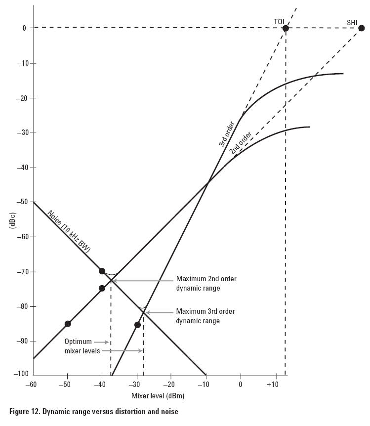
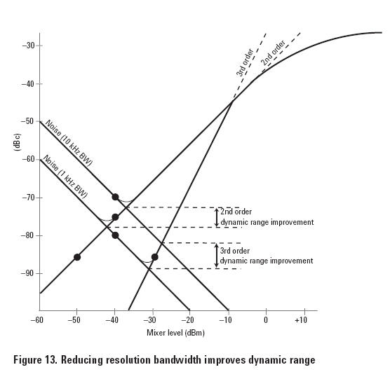
Hint 4. Optimize Dynamic Range When Measuring Distortion

An issue that comes up with measuring signals is the ability to distinguish the larger signal’s fundamental tone signals from the smaller distortion products. The maximum range that a spectrum analyzer can distinguish between signal and distortion, signal and noise, or signal and phase noise is specified as the spectrum analyzer’s dynamic range.  When measuring signal and distortion, the mixer level dictates the dynamic range of the spectrum analyzer. The mixer level used to optimize dynamic range can be determined from the second-harmonic distortion, third fundamental at the mixer, the SHD increases 2 dB. However, since distortion is determined by the difference between fundamental and distortion product, the change is  only 1 dB. Similarly, the third-order distortion is drawn with a slope of 2. For every 1 dB change in mixer level, 3rd order products change 3 dB, or 2 dB in a relative sense.  The maximum 2nd and 3rd order dynamic range can be achieved by setting the mixer at the level where the 2nd and 3rd order distortions are equal to the noise floor, and these mixer levels are identified in the graph. order intermodulation distortion,  and displayed average noise level  (DANL) specifications of the spectrum  analyzer. From these specifications, a graph of internally generated distortion and noise versus mixer level can be made.  Figure 12 plots the -75 dBc second harmonic distortion point at -40 dBm mixer level, the -85 dBc third-order distortion point at a -30 dBm mixer level and a noise floor of -110 dBm for a 10 kHz RBW.

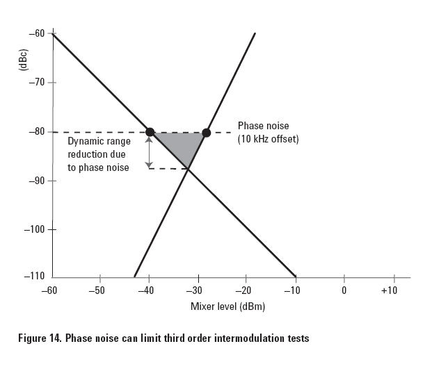
The second harmonic distortion line is drawn with a slope of 1 because for each 1 dB increase in the level of the fundamental at the mixer, the SHD  increases 2 dB. However, since distortion is determined by the difference between fundamental and distortion product, the change is only 1 dB. Similarly, the third-order distortion is drawn with a slope of 2. For every 1 dB change in mixer level, 3rd order products change 3 dB, or 2 dB in a relative sense.  The maximum 2nd and 3rd order dynamic range can be achieved by setting the mixer at the level where the 2nd and 3rd order distortions are equal to the noise floor, and these mixer levels are identified in the graph.  To increase dynamic range, a narrower resolution bandwidth must be used. The dynamic range increases when the RBW setting is decreased from 10 kHz to 1 kHz as showed in Figure 13. Note that the increase is 5 dB for 2nd order and 6+ dB for 3rd order distortion.  Lastly, dynamic range for intermodulation distortion can be affected by the phase noise of the spectrum analyzer because the frequency spacing between the various spectral components (test tones and distortion  products) is equal to the spacing  between the test tones. For example, test tones separated by 10 kHz, using a 1 kHz resolution bandwidth sets the noise curve as shown. If the phase noise at a 10 kHz offset is  only -80 dBc, then 80 dB becomes  the ultimate limit of dynamic range  for this measurement, instead of a  maximum 88 dB dynamic range as  shown in Figure 14.   

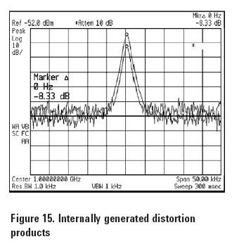
Hint 5. Identifying Internal Distortion Products

High-level input signals may cause internal spectrum analyzer distortion products that could mask the real distortion on the input signal.  Using dual traces and the analyzer’s RF attenuator, you can determine whether or not distortion generated within the analyzer has any effect on the measurement.  To start, set the input attenuator so that the input signal level minus the attenuator setting is about -30 dBm.  To identify these products, tune to the second harmonic of the input signal and set the input attenuator to 0 dBm. Next, save the screen data in Trace B, select Trace A as the active trace, and activate Marker Ä.  The spectrum analyzer now shows the stored data in Trace B and the measured data in Trace A, while Marker Ä shows the amplitude and frequency difference between the two traces. Finally, increase the RF attenuation by 10 dB and compare the response in Trace A to the response in Trace B. 

If the responses in Trace A and Trace B differ, as in Figure 15, then the spectrum analyzer’s mixer is generating internal distortion products due to  the high level of the input signal. In this case, more attenuation is required. 

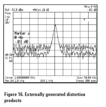
In Figure 16, since there is no change in the signal level, the internally generated distortion has no effect on the measurement.  The distortion that is displayed is present on the input signal. 

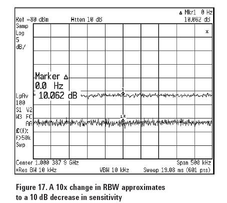
Hint 6. Optimize Measurement Speed When Measuring Transients

Fast sweeps are important for capturing transient signals and minimizing test time. To optimize the spectrum analyzer performance for faster sweeps, the parameters that determine sweep time must be changed accordingly.  Sweep time for a swept-tuned superheterodyne spectrum analyzer is approximated by the span divided by the square of the resolution bandwidth (RBW). Because of this, RBW settings largely dictate the sweep time. Narrower RBW filters translate to longer sweep times, which translate to a tradeoff between sweep speed and sensitivity. As shown in Figure 17, a 10x change in RBW approximates to a 10 dB improvement in sensitivity.

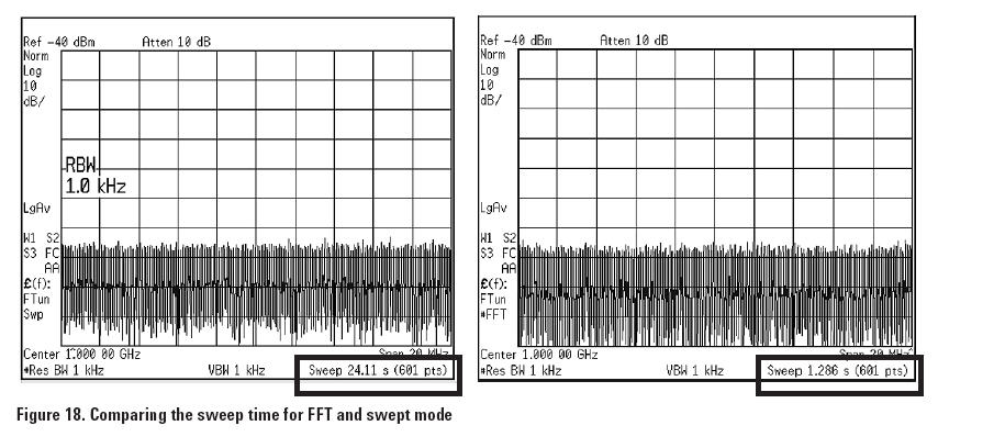
Depending on the use, the modern high-performance spectrum analyzer RBW can be decreased (in fine  steps) to meet the necessary sweep  speed, sensitivity and/or selectivity.  Figure 2 shows a 7.626 s sweep speed for a 10 kHz RBW compared to 26.79 s for a 3 kHz RBW setting shown in Figure 3.  A good balance between time and sensitivity is to use fast fourier transform (FFT) that is available in the modern high-performance spectrum analyzers. By using FFT, the analyzer is able to capture the entire span in one measurement cycle.  When using FFT analysis, sweep time is dictated by the frequency span instead of the RBW setting.  Therefore, FFT mode proves shorter sweep times than the swept mode in narrow spans. The difference in speed is more pronounced when the RBW filter is narrow when measuring low-level signals. In the FFT mode, the sweep time for a 20 MHz span and 1 kHz RBW is 747.3 ms compared to 24.11 s for the swept mode as shown in Figure 18 below.  For much wider spans and wide RBW’s, swept mode is faster.     

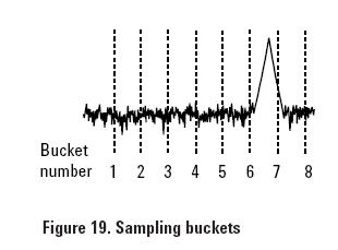
Hint 7. Selecting the Best Display Detection Mode

Modern spectrum analyzers digitize the signal either at the IF or after the video filter. The choice of which digitized data to display depends on the display detector following the ADC. It is as if the data is separated into buckets, and the choice of which data to display in each bucket becomes affected by the display detection mode.

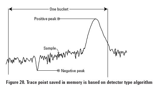
Positive peak, negative peak and sample detectors are shown in Figure 20.

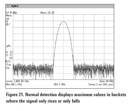
Peak detection mode detects the highest level in each bucket, and is a good choice for analyzing sinusoids, but tends to over-respond to noise. It is the fastest detection mode.  Sample detection mode displays the center point in each bucket, regardless of power. Sample detection is good for noise measurements, and accurately indicates the true randomness of noise. Sample detection, however, is inaccurate for measuring continuous wave (CW) signals with narrow resolution bandwidths, and may miss signals that do not fall on the same point in each bucket.  Negative peak detection mode displays the lowest power level in each bucket. This mode is good for AM or FM demodulation and distinguishes between random and impulse noise.  Negative peak detection does not give the analyzer better sensitivity, although the noise floor may appear to drop. A comparative view of what each detection mode displays in a bucket for a sinusoid signal is shown in Figure 20.  Higher performance spectrum analyzers also have a detection mode called Normal detection, shown in Figure 21.

This sampling mode dynamically classifies the data point as either noise or a signal, providing a better visual display of random noise than peak detection while avoiding the missed-signal problem of sample detection.  Average detection can provide the average power, voltage or log-power (video) in each bucket. Power averaging calculates the true average power, and is best for measuring the power of complex signals. Voltage averaging averages the linear voltage data of the envelope signal measured during the bucket interval. It is often used in EMI testing, and is also useful for observing rise and fall behavior of AM or pulse-modulated signals such as radar and TDMA transmitters. Log-power (video) averaging averages the logarithmic amplitude values (dB) of the envelope signal measured during the bucket interval. Log power averaging is best for observing sinusoidal signals, especially those near noise because noise is displayed 2.5 dB lower than its true level and improves SNR for spectral (sinusoidal) components.

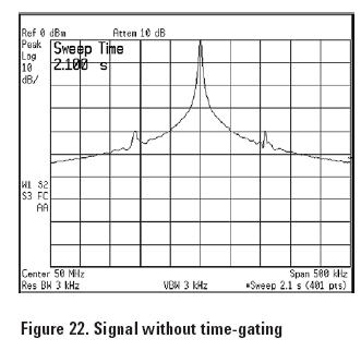
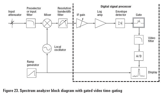
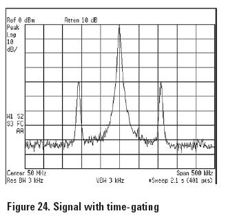
Hint 8. Measuring Burst Signals: Time Gated Spectrum Analysis

How do you analyze a signal that consists of a burst (pulsed) RF carrier that carries modulation when pulsed on? If there is a problem, how do you separate the spectrum analysis of the pulse from that of the modulation?  Analyzing burst signals (pulses)  with a spectrum analyzer is very  challenging because in addition to  displaying the information carried  by the pulse, the analyzer displays  the frequency content of the shape  of the pulse (pulse envelope) as well.  The sharp rise and fall times of the pulse envelope can create unwanted frequency components that add to the frequency content of the original signal. These unwanted frequency components might be so bad that they completely obscure the  signal of interest.  Figure 22, for example, depicts the frequency content of a pulse carrying a simple AM signal. In this case, the AM sidebands are almost completely hidden by the pulse spectrum.

Time gated spectral analysis permits analysis of the contents of the pulse without the effect of the envelope of the pulse itself. One way of performing time-gating is to place a gate (switch) in the video path of the spectrum analyzer as shown in Figure 23.  This method of time-gating is called gated video.  In a time gated measurement, the analyzer senses when the burst starts, then triggers a delay so the resolution filter has time to react to the sharp rise time of the pulse, and finally stops the analysis before the burst ends. By doing this, only the information carried by the pulse is analyzed, as is shown in Figure 24.  It is now clear that our pulse contained a 40 MHz carrier modulated by a 100 kHz sinusoidal signal.  Two other types of time-gating available in the modern highperformance spectrum analyzer are gated-LO and gated-FFT. Gated-LO sweeps the local oscillator during part of the pulsed signal so several trace points can be recorded for each occurrence of the signal.  Whereas gated-FFT takes an FFT of the digitized burst signal removing the effect of the pulse spectrum.  Both provide advantages of increased speed.

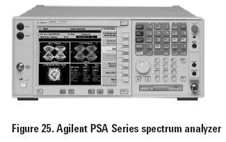
Agilent PSA Series Spectrum Analyzer

These spectrum analyzers offer highperformance spectrum analysis up  to 50 GHz, with powerful one-button  measurements, a versatile feature  set, and a leading-edge combination  of flexibility, speed, accuracy, analysis  bandwidth, and dynamic range.  From millimeter wave and phase noise, noise figure measurements to  spur searches and digital modulation  analysis, the PSA Series provides  unique and comprehensive  solutions to R&D and manufacturing  engineers in cellular and emerging  wireless communications, aerospace,  and defense.

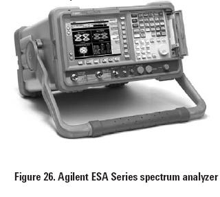
Agilent ESA Series Spectrum Analyzer

The ESA Series spectrum analyzers provide scalable basic and midperformance spectrum analysis, for general-purpose or application focused measurements from cellular  communications to wireless networking  to cable TV. The ESA is available as an Express Analyzer with atwo-week availability and are value priced.

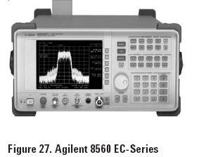
Agilent 8560 EC-Series Spectrum Analyzer

Providing high performance, capability, and quality for the most demanding measurements, these spectrum analyzers have the  performance and features you  require on the R&D bench.  With the reliability and speed you depend upon in production and the ease-of-use, portability, and MIL ruggedness you expect in the field,  these spectrum analyzers will meet your high  performance needs.

Related Spectrum Analyzer and Spectrum Analysis Literature

Spectrum Analysis Basics, Application Note 150, literature number 5952-0292

Optimizing Spectrum Analyzer Measurement Speed, Application Note 1318, literature number 5968-3411E

Optimizing Dynamic Range for Distortion Measurements, Product Note, literature number 5980-3079EN

Optimizing Spectrum Analyzer Amplitude Accuracy, Application Note 1316, literature number 5968-3659E

Selecting the Right Signal Analyzer for Your Needs, Selection Guide, literature number 5968-3413E

PSA Series Swept and FFT Analysis, Product Note, literature number 5980-3081EN